Project 2: Fun with Filters and Frequencies
Overview
This project explores various image processing techniques, including sharpening, gradient-based edge detection, and hybrid image blending. Through the use of filters and frequency transformations, I manipulate images to highlight features and create visual effects that range from sharpening details to blending multiple images at different resolutions.
Part 1.1: Finite Difference Operators
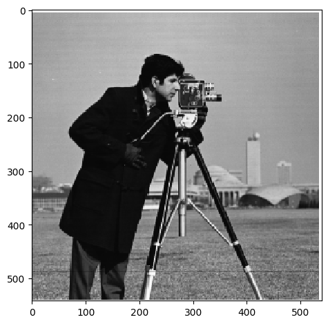
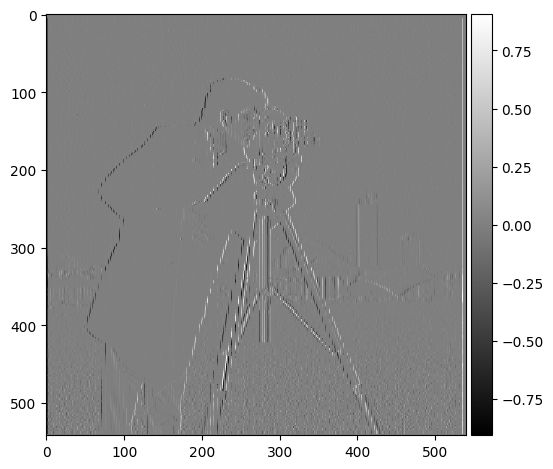
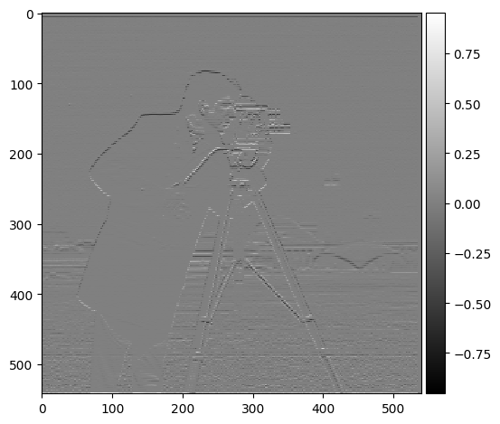
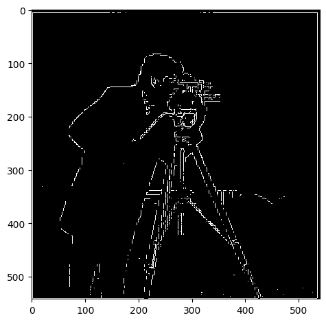
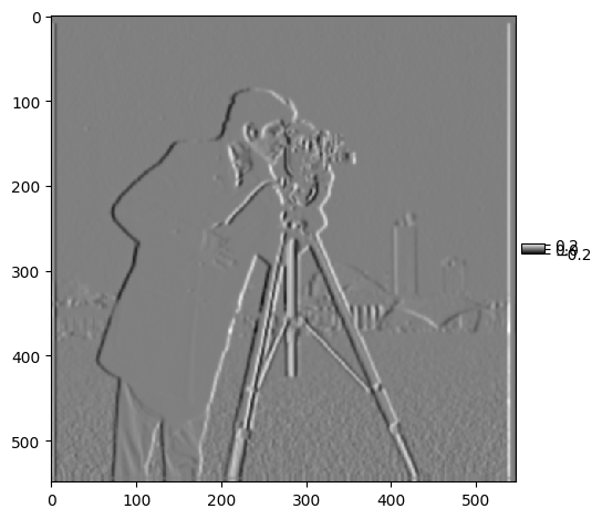
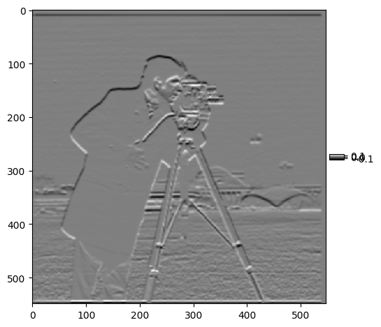
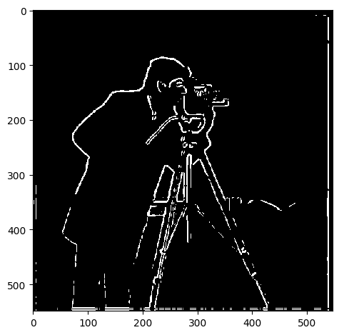
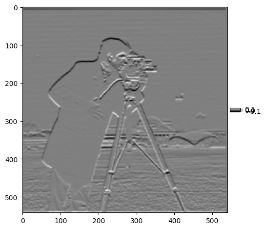
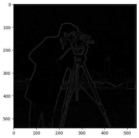
In this part, I calculated the partial derivatives of the image in both the x and y directions by convolving the image with finite difference operators Dx and Dy. This convolution highlights changes in pixel intensity along each axis, which helps to identify edges in the image. After computing the gradient magnitudes, I generated an edge image by binarizing the gradient magnitude using a threshold, 0.3. This threshold was selected to minimize noise while preserving important edges. Below are the results:

Original Image

Grad X

Grad Y

Gradient Magnitude

Binarized Gradient Magnitude
Part 1.2: Derivative of Gaussian (DoG) Filter
In this part, I aimed to reduce the noise observed in the previous section by applying a Gaussian filter before computing the finite differences. The Gaussian filter smooths the image by blurring it, which helps to reduce the noise caused by the finite difference operators. Below are the results after convolving the blurred image with the finite difference operators to compute the gradient in the x and y directions, followed by calculating the gradient magnitude and binarizing it:

Grad X

Grad Y

Gradient Magnitude

Binarized Gradient Magnitude
By comparing these results with those from Part 1, it's clear that the application of the Gaussian filter significantly reduces noise, resulting in more distinct and solid edges. The edges in this version appear less fragmented and noisy compared to the results using the raw finite difference operators alone.
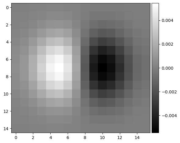
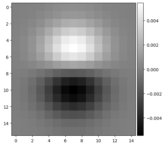
Next, I combined the Gaussian filter and the finite difference operator in one step by computing the Derivative of Gaussian (DoG) filters. This allows for a single convolution instead of two. Below are the images for the DoG filters in the x and y directions, as well as the computed gradient magnitudes:

DoGx

DoGy

Gradient DogX

Gradient DogY

Dog Gradient Magnitude

Dog Binarized Gradient Magnitude
The results produced by the DoG filters are nearly identical to those obtained by first applying the Gaussian blur and then using finite differences. This demonstrates that combining these steps into a single convolution achieves the same outcome while improving computational efficiency.
Part 2.1: Sharpening Images
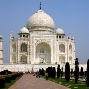
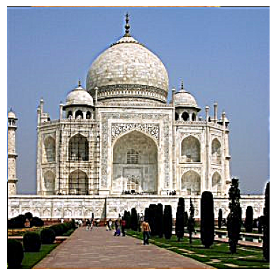
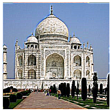
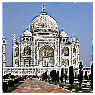
In this part, I applied the unsharp masking technique to sharpen various images. The idea behind unsharp masking is to enhance the high-frequency details of an image, which are often perceived as sharpness. This is done by first applying a Gaussian blur to the image, which acts as a low-pass filter that removes the high-frequency details. By subtracting the blurred image from the original, we isolate the high-frequency components. We then add back a scaled version of these high frequencies to the original image, enhancing the sharpness.
Results on the Taj Mahal Image:

Original Image

Sharpened Image (Alpha = 2)

Sharpened Image (Alpha = 5)

Sharpened Image (Alpha = 10)
As we increase the alpha value, the image becomes progressively sharper, but higher alpha values can also introduce some artifacts or make the image look overly processed. For example, at Alpha = 10, the image appears significantly sharper, but some of the natural details may be exaggerated.
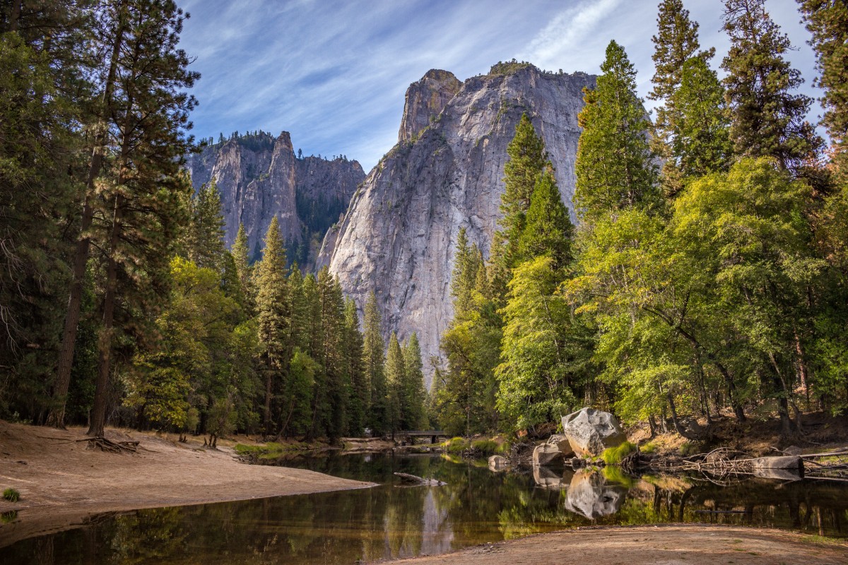
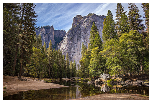
Results on the Mountain Image:

Original Image

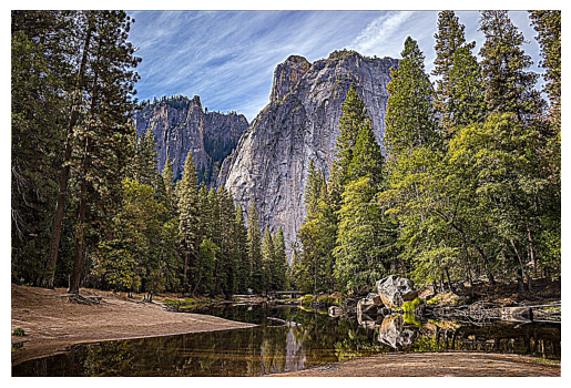
Sharpened Image (Alpha = 2)

Sharpened Image (Alpha = 5)

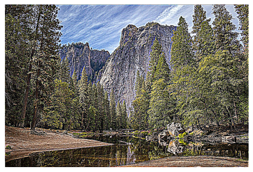
Sharpened Image (Alpha = 10)
Similar to the Taj Mahal image, the mountain image shows noticeable sharpening with higher alpha values. However, the textures of natural features like rocks and trees may appear overly enhanced at higher alpha settings.
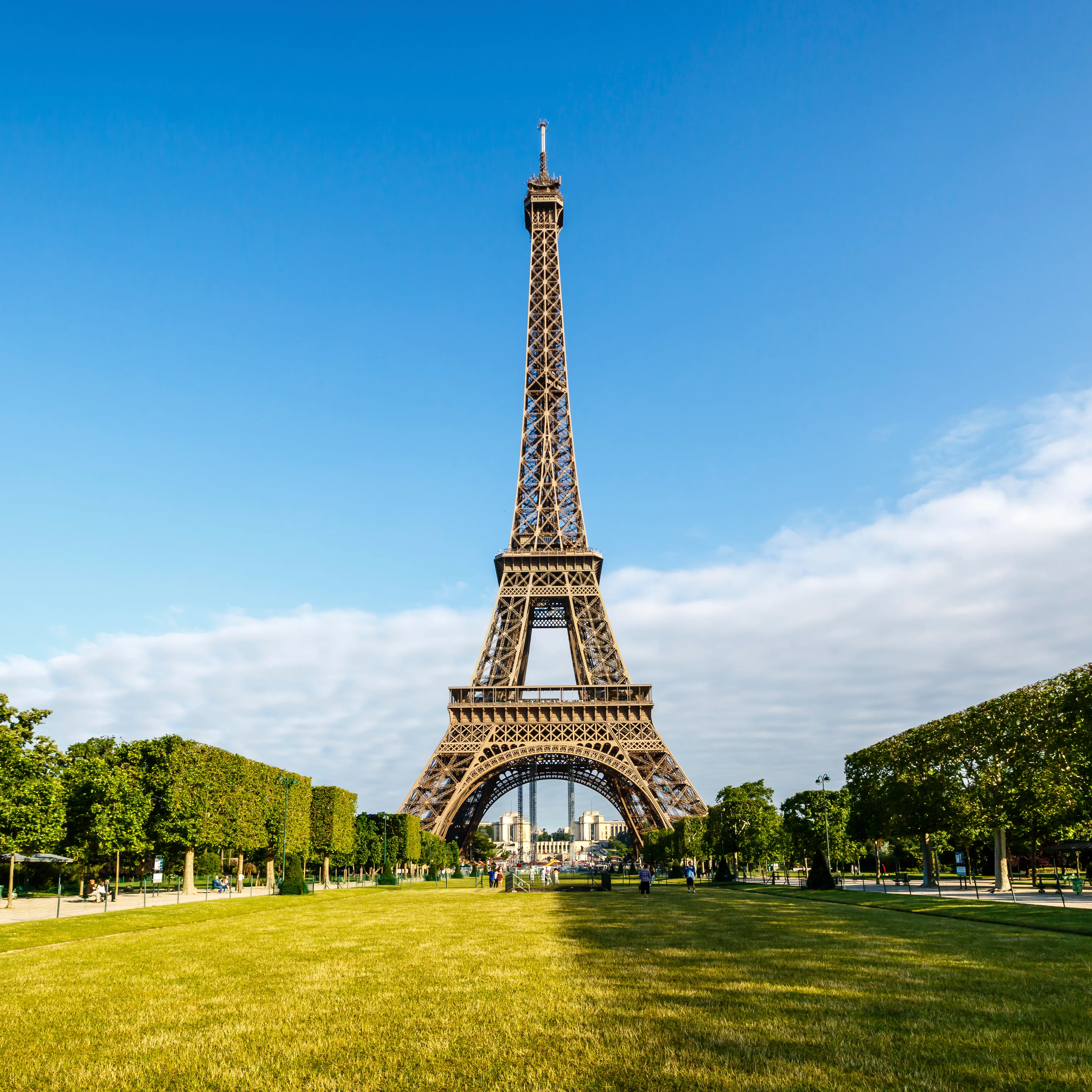
Resharpening a Blurred Image (Eiffel Tower):
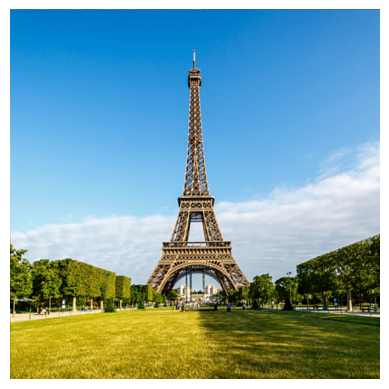
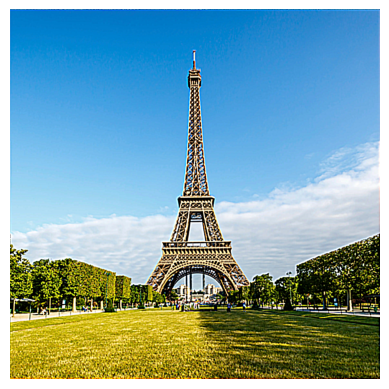
I took a sharp image of the Eiffel Tower, applied a Gaussian blur to it, and then attempted to restore its sharpness using the unsharp masking technique.

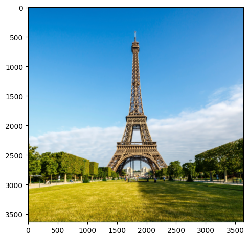
Original Image

Blurred Image

Resharpened Image (Alpha = 2)

Resharpened Image (Alpha = 10)
After applying the blur and then attempting to sharpen the image again, we can see that some sharpness is restored. However, since the high-frequency details are lost during the initial blur, the sharpened result doesn't fully recover the original level of detail.
Part 2.2: Hybrid Images
In this part, I created hybrid images by combining the high-frequency details of one image with the low-frequency details of another. The concept behind hybrid images is that they appear differently when viewed up close versus at a distance. At close range, high-frequency details dominate, whereas, at a distance, only the low-frequency components are visible.
Example 1: Hybrid Image of Nutmeg and Derek
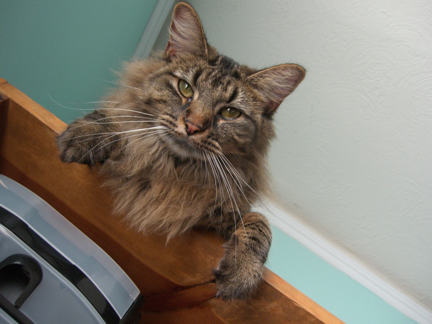
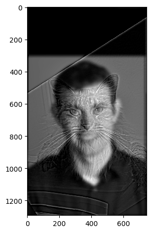
The high-frequency components from Nutmeg were combined with the low-frequency components from Derek. The result is a hybrid image that looks like Nutmeg from up close but transitions into Derek’s face when viewed from far away.

Nutmeg (Low Frequency)

Derek (High Frequency)

Hybrid Image (DerNut)
Frequency Domain Analysis for Nutmeg and Derek
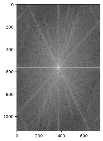
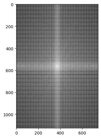
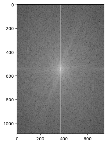
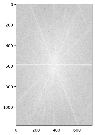
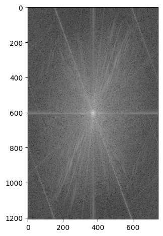
I performed a Fourier transform on the images to analyze their frequency components. The log magnitude of the Fourier transform shows how much each frequency contributes to the overall image. The low-pass filtered version of Derek keeps only the low-frequency information, while the high-pass filtered Nutmeg emphasizes the high-frequency details.

FFT of Derek

Lowpass Filtered Derek

FFT of Nutmeg

Highpass Filtered Nutmeg

Hybrid Image
Example 2: Expression Change of Kamala
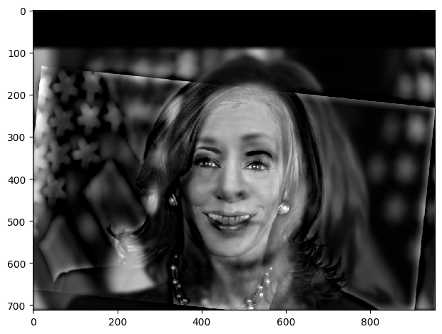
In this example, I created a hybrid image by blending two facial expressions of the same person: one with a neutral expression and one with a smile. The low-frequency components of the neutral face are combined with the high-frequency components of the smiling face. From a distance, the image looks neutral, but as you move closer, the smile becomes more apparent.

Smile (High Frequency)

Neutral (Low Frequency)

Hybrid Image (Smile/Neutral)
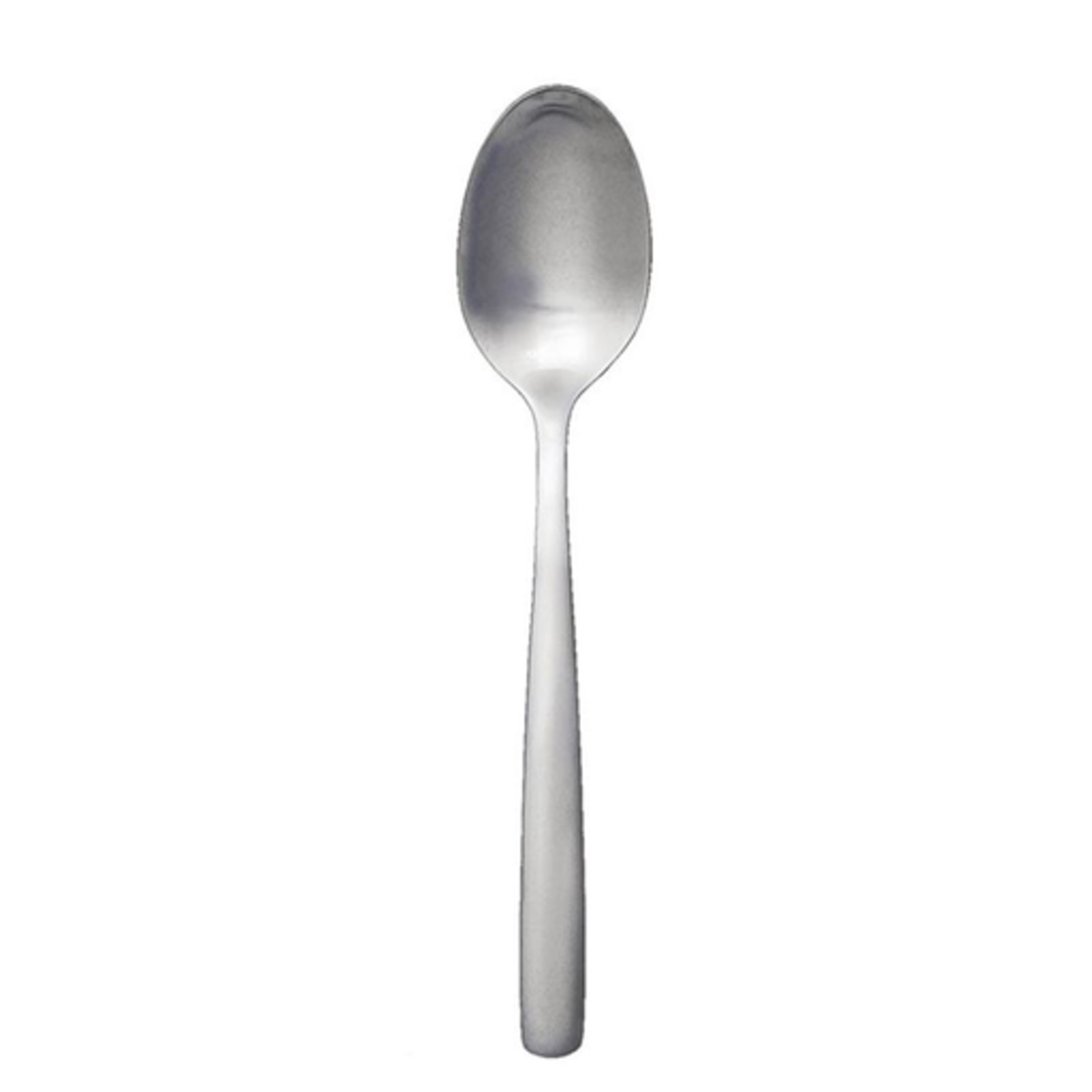
Example 3: Failed Morph Between Objects - Fork and Spoon
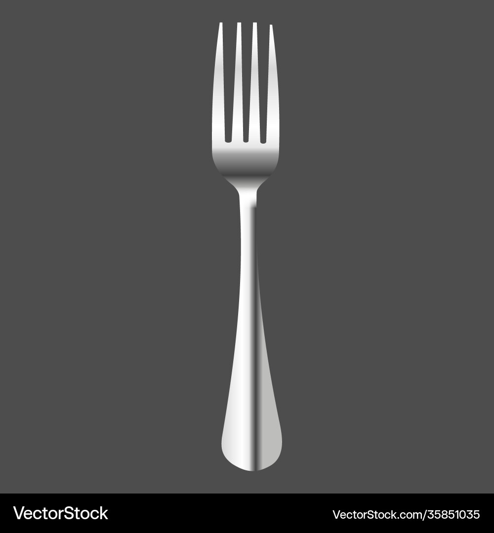
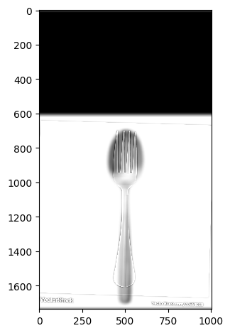
I attempted to create a spork. A fork from up close but a spoon from afar. However, the results weren't what I expected. The fork appears invisible. I believe this is because there is too much overlap of the same color. Causing the fork to become invisible or ghostly. I attempted playing with the background using a grey and white background for the fork. However, there was no success. I additionally played with the lowpass and highpass sigma values, however it never fixed the issue of the spoon overpowering the invisible fork.

Fork (High Frequency)

Spoon (Low Frequency)

Hybrid Image (Spork)
Part 2.3: Gaussian and Laplacian Stacks
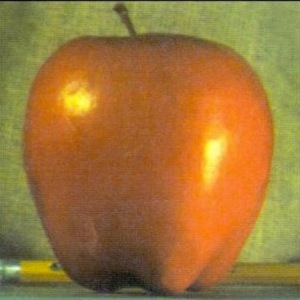
In this part, I implemented Gaussian and Laplacian stacks, which are used for multi-resolution image blending. The Gaussian stack captures progressively smoother versions of the image by repeatedly applying Gaussian filters at each level without downsampling.
Gaussian Stack

Gaussian Stack: Apple

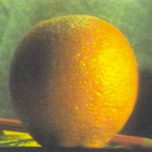
Gaussian Stack: Orange
Laplacian Stack
The Laplacian stack captures details lost between consecutive levels of the Gaussian stack. By subtracting the Gaussian blurred image at one level from the next level, we isolate the band-pass features, effectively capturing the details that lie between high and low-frequency components.

Laplacian Stack: Apple

Laplacian Stack: Orange
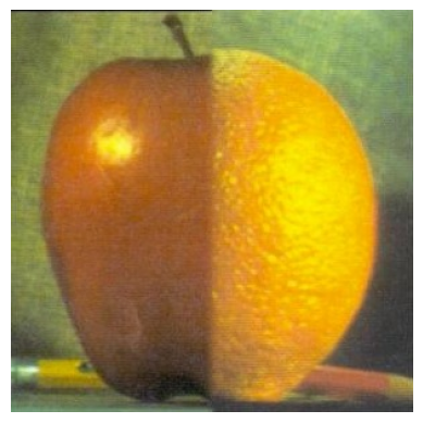
Part 2.4: Multiresolution Blended Images
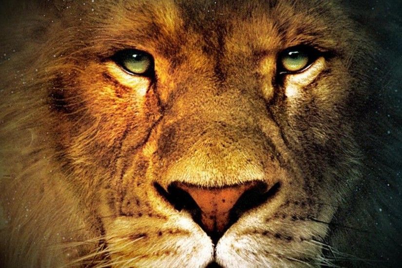
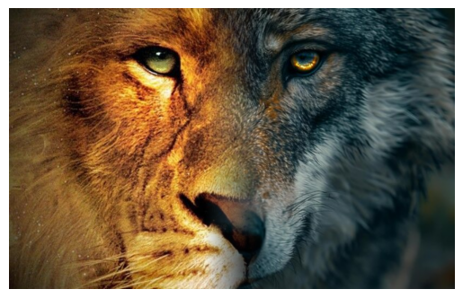
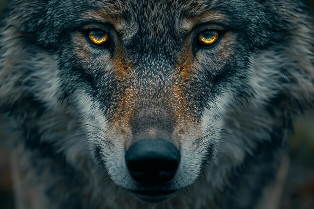
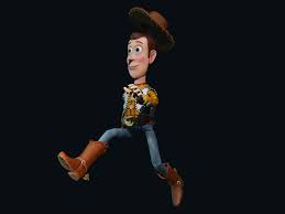
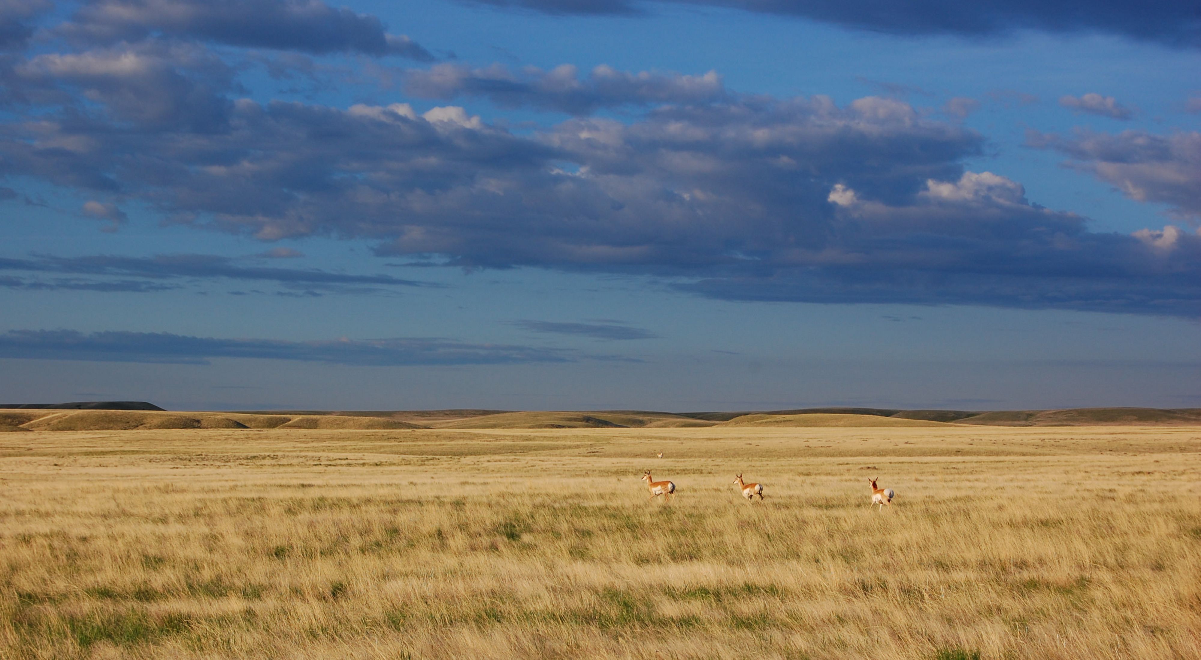
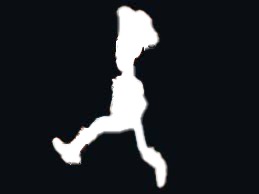
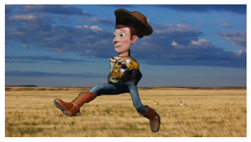
Here I used a variety of masks to combine images. The first example uses the part above and is the final result of the blur. The image between two animals was slightly more complex as I had to use a smoother blur to combine it changing the mask. The final example shows a custom mask. I used an AI cropper in Photoshop to create a layer on the original Woody image to create a black and white mask. I then overlayed this with the image and using the same stack procedure as before I put Woody in the Plains.

Lion

Winter/Summer King

Wolf

Woody

Plains

Mask

Woody in the Plains

Laplacian Stack Wolf

Laplacian Stack Lion
